Optimal binary search trees
Suppose that we are designing a program to translate text from English to French. For each occurrence of each English word in the text, we need to look up its French equivalent. We could perform these lookup operations by building a binary search tree with $n$ English words as keys and their French equivalents as satellite data. Because we will search the tree for each individual word in the text, we want the total time spent searching to be as low as possible. We could ensure an $Θ(log_2 \;n)$ search time per occurrence by using a red-black tree or any other balanced binary search tree. Words appear with different frequencies, however, and a frequently used word such as the may appear far from the root while a rarely used word appears near the root. Such an organization would slow down the translation, since the number of nodes visited when searching for a key in a binary search tree equals one plus the depth of the node containing the key. We want words that occur frequently in the text to be placed nearer the root. How do we organize a binary search tree so as to minimize the number of nodes visited in all searches, given that we know how often each word occurs? [1]
What we need is known as an optimal binary search tree. Formally, we are given a sequence $K = (k_1, k_2 \cdots k_n)$ of $n$ distinct keys in sorted order (so that $k_1 \lt k_2 \lt \cdots \lt k_n$), and we wish to build a binary search tree from these keys. For each key $k_i$, we have a probability $p_i$ that a search will be for $k_i$. Some searches may be for values not in $K$, and so we also have $n + 1$ dummy keys $d_0, d_1 \cdots d_n$ representing values not in $K$. For each dummy key $d_i$, we have a probability $q_i$ that a search will correspond to $d_i$ [1]. The probability table is given below. [1]
$$
\begin{array}{c|ccc}
i & \text{0} & \text{1} & \text{2} & \text{3} & \text{4} & \text{5}\\
\hline
p_i & & 0.15 & 0.10 & 0.05 & 0.10 & 0.20 \\
q_i & 0.05 & 0.10 & 0.05 & 0.05 & 0.05 & 0.10
\end{array}
$$
Based on the above observation, we can derive the equation:
$$
\sum_{i=1}^n p_i + \sum_{i=0}^n q_i = 1
$$
Now we can determine the expected cost of a search in a given binary search tree $T$. Let us assume that the actual cost of a search equals the number of nodes examined. Then the expected cost of a search in $T$ is given by [1]:
$$
E[search \;cost\; in\; T] = \sum_{i=1}^n (depth_T(k_i)+1).p_i + \sum_{i=0}^n (depth_T(d_i)+1).q_i \\
= 1 + \sum_{i=1}^n depth_T(k_i).p_i + \sum_{i=0}^n depth_T(d_i).q_i
$$
For a given set of probabilities, we wish to construct a binary search tree whose expected search cost is smallest. We call such a tree an optimal binary search tree. Exhaustive checking of all possibilities fails to yield an efficient algorithm. We can prove that the number of binary trees with $n$ nodes is $\Omega(4^n/n^{3/2})$ and so we would have to examine an exponential number of binary search trees in an exhaustive search. Not surprisingly, we shall solve this problem with dynamic programming. [1]
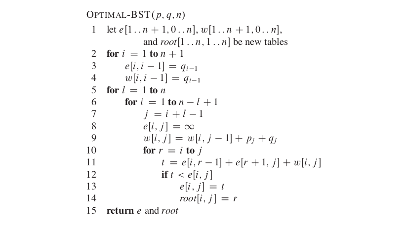
We are ready to define the value of an optimal solution recursively. We pick our subproblem domain as finding an optimal binary search tree containing the keys $k_i \cdots k_j$ where $i \ge 1,\; j \le n$ and $j \;\ge i - 1$. Let us define $e[i, j]$ as the expected cost of searching an optimal binary search tree containing the keys $k_i \cdots k_j$.
The trivial case occurs when $j = i - 1$, Then we have just the dummy key $d_{i - 1}$. The expected search cost is thus, $e[i, i-1] = q_{i-1}$
When $j \ge i$, we need to select a root $k$r from among $k_i \cdots k_j$ and then make an optimal binary search tree with keys $k_i \cdots k_{r-1}$ as its left subtree and an optimal binary search tree with keys $k_{r+1} \cdots k_j$ as its right subtree. [1]
By equation above, the expected search cost of this subtree increases by the sum of all the probabilities in the subtree when it becomes a subtree of a node.
$$
w(i, j)=\sum_{l=i}^j p_l + \sum_{l=i-1}^j q_l
$$
Thus, if $k_r$ is the root of an optimal subtree containing keys $k_i \cdots k_j$, we have
$$e[i, j] = p_r + (e[i, r-1] + w[i, r-1]) +(e[r+1, j] + w[r+1, j])$$
Note that,$$w[i, j] = w[i, r-1] + p_r + w[r+1, j]$$
And we rewrite $e[i, j]$ as, $$e[i, j] = e[i, r-1] + e[r+1, j] + w[i, j]$$
We choose the root that gives the lowest expected search cost, giving us our final recursive formulation:
$\large length[i][j] =
\begin{cases}
q_{i-1} , & \text{if $j = i-1$} \\[2ex]
\min_{\forall r \;such\;that\; i\le r \le j}\left\{e[i, r-1] + e[r+1, j] + w[i, j]\right\}, & \text{if $i \le j $}
\end{cases}$
To help us keep track of the structure of optimal binary search trees, we define $root[i, j]$, for $1 \le i \le j \le n$, to be the index $r$ for which $k_r$ is the root of an optimal binary search tree containing keys $k_i \cdots k_j$. [1]
Exercise 15.5-1
Write pseudocode for the procedure CONSTRUCT-OPTIMAL-BST(root) which, given the table root, outputs the structure of an optimal binary search tree. Your procedure should print out the structure [1]
$k_2$ is the root
$k_1$ is the left child of $k_2$
$d_0$ is the left child of $k_1$
$d_1$ is the right child of $k_1$
$k_5$ is the right child of $k_2$
$k_4$ is the left child of $k_5$
$k_3$ is the left child of $k_4$
$d_2$ is the left child of $k_3$
$d_3$ is the right child of $k_3$
$d_4$ is the right child of $k_4$
$d_5$ is the right child of $k_5$
Answer:
$CONSTRUCT-OPTIMAL-BST(root)$
$\phantom{{}++{}}$ $n \gets root.length$
$\phantom{{}++{}}$ $r \gets root[1][n]$
$\phantom{{}++{}}$ `print` $k_r$ is the root
$\phantom{{}++{}}$ $CONSTRUCT-OPTIMAL-BST-AUX(root, 1, r - 1, r, left)$
$\phantom{{}++{}}$ $CONSTRUCT-OPTIMAL-BST-AUX(root, r + 1, n, r, right)$
$CONSTRUCT-OPTIMAL-BST-AUX(root, i, j, p, s)$
$\phantom{{}++{}}$ `if` $i \le j$
$\phantom{{}++{}}$ $\phantom{{}++{}}$ $r \gets root[i][j]$
$\phantom{{}++{}}$ $\phantom{{}++{}}$ `print` $k_r$ is the $\langle s \rangle$ child of $k_p$
$\phantom{{}++{}}$ $\phantom{{}++{}}$ $CONSTRUCT-OPTIMAL-BST-AUX(root, i, r - 1, r, left)$
$\phantom{{}++{}}$ $\phantom{{}++{}}$ print $d_j$ is the $\langle s \rangle$ child of $k_p$
And here’s the code:
Comments
Post a Comment